
Tutorial: Building A Basic Home Budget Spreadsheet In Excel (For Beginners)
This website may earn commissions from purchases made through links in this post. As an Amazon Associate, I earn from qualifying purchases.
Creating your own basic home budget spreadsheet in Excel is a great way to get a hold on your spending patterns and overall financial health and knowing your way around Excel is a handy skill to have.

Excel is an awesome program for personal budgeting. I have been using it now for over a decade.
When you create your own budget yourself, you can customise it to meet your own needs and circumstances exactly.
This tutorial starts from the very beginning for those who have never met a spreadsheet before.
The tutorial is based on the latest version of Excel, so if you’re using the older version of Excel, you will find the same functions in the toolbar and menu bar.
If you don’t have Excel, then the free alternatives (Open Office or Google spreadsheets) are pretty similar and this tutorial should still be helpful the functions will just be in different menus.
Disclaimer: This is general information only. In this blog, I share my savings and budget planning and what works for us, linking to authority websites where relevant. You should always consult a qualified financial expert when making money decisions to tailor plans to suit your circumstances.
Steps Building A Basic Home Budget Spreadsheet
Below are the steps, accompanied with diagrams, to creating a basic home budget.
Make sure to customise the spreadsheet expense and income categories to your personal circumstances.
1. Set Up Your Spreadsheet Budget
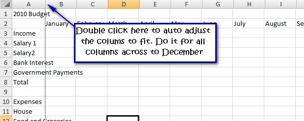
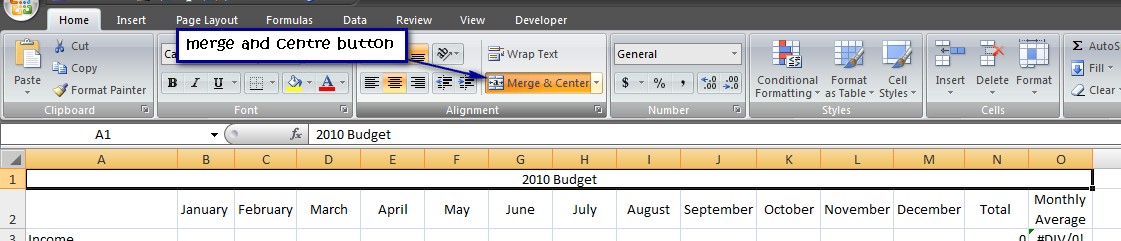
Start a new document and give it a heading like [Year] Budget.
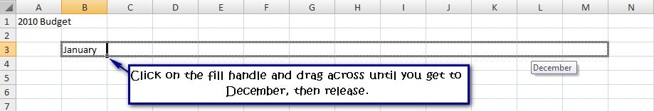
Next, type the months along the next row, staring at B2.
Tip: if you type January and click on the small black box (fill handle) in the bottom right-hand corner of cell B2 and drag it across, it will fill in the rest of the months for you without you having to type them.
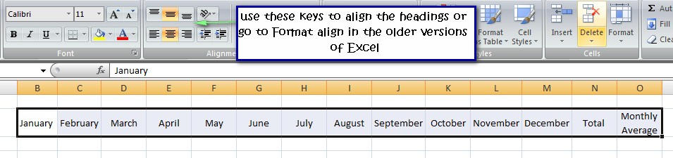
After December, type the headings Total and Monthly Average.

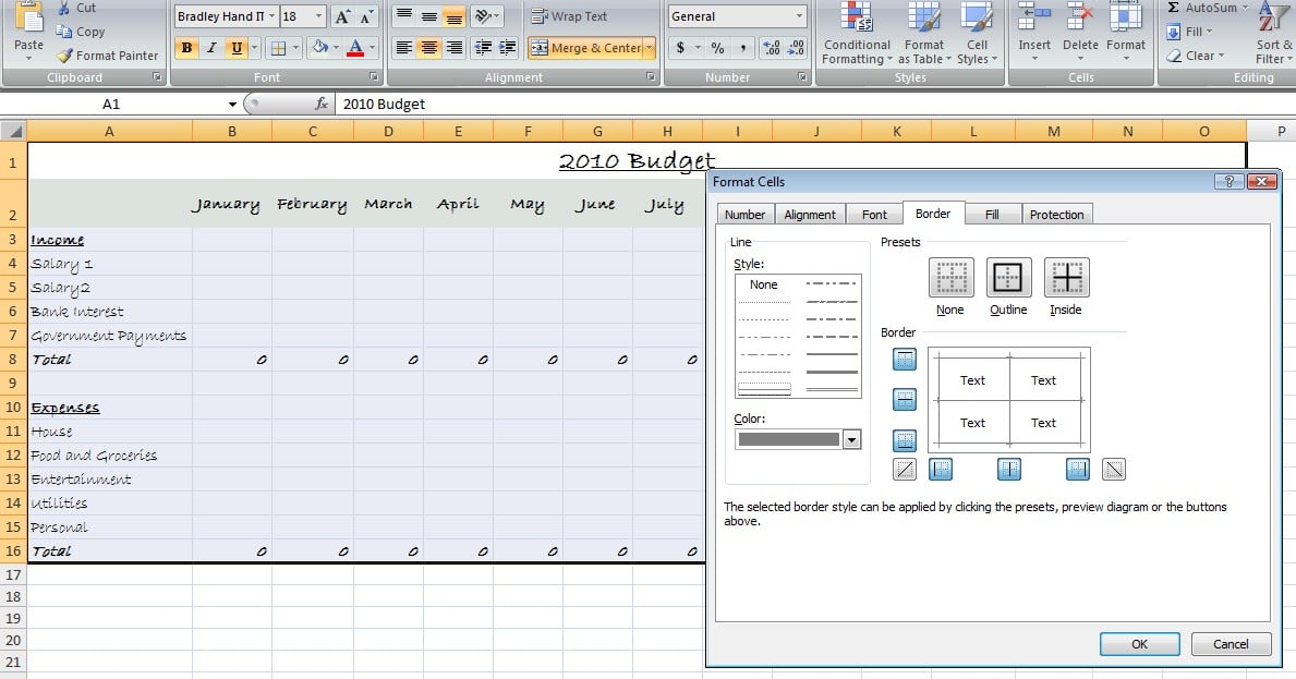
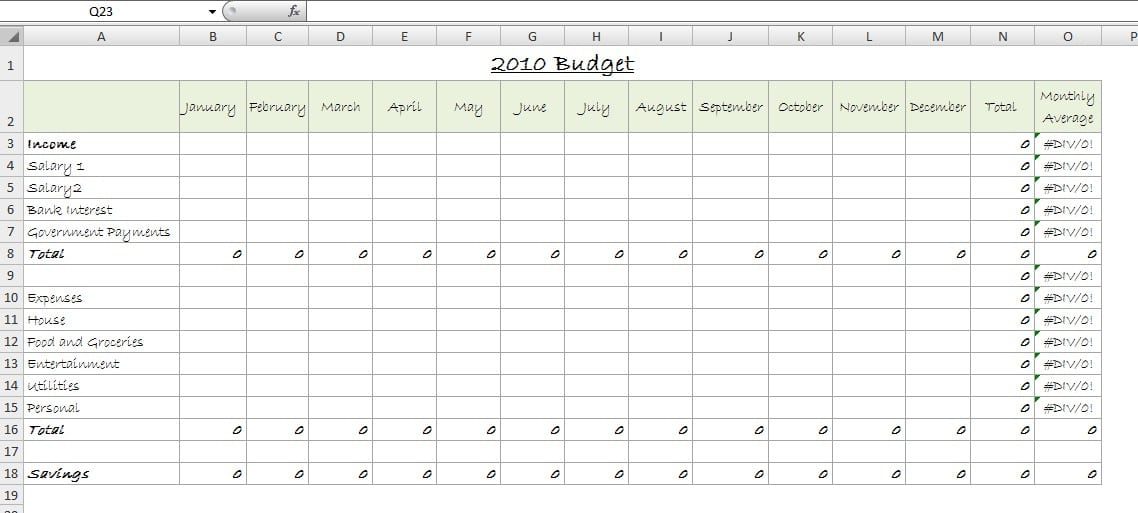
In A3 type the heading Income and list below all streams of income followed by a Total row as shown below.
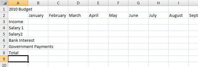
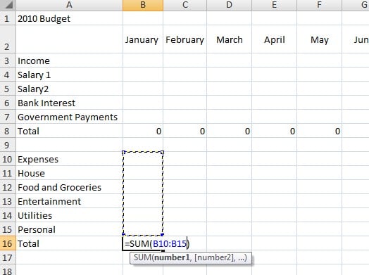
Skip a row and type the heading Expenses in A10 and list all expense categories followed by a Total row.
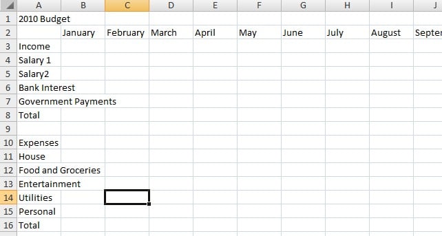
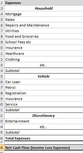
I’ve just typed in a few basic categories for the sake of example, type in as many categories as are relevant to you. You may prefer to set out more specific expense categories, something like this:
Double click the line between each column to automatically adjust the columns to fit the content.
For the Monthly Average heading, click in the cell and select wrap text. This should automatically adjust the height of row 2, but if it doesn’t, click and drag the line between row 2 and 3 to adjust the height to fit the heading.
Select the cells January to Monthly Average (when selecting cells, your cursor should look like a white cross) and centre them vertically and horizontally.
2. Enter Formulas to Calculate Your Budget
The next step is to enter your formulas. This makes your budget calculate automatically.
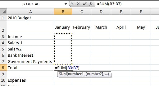
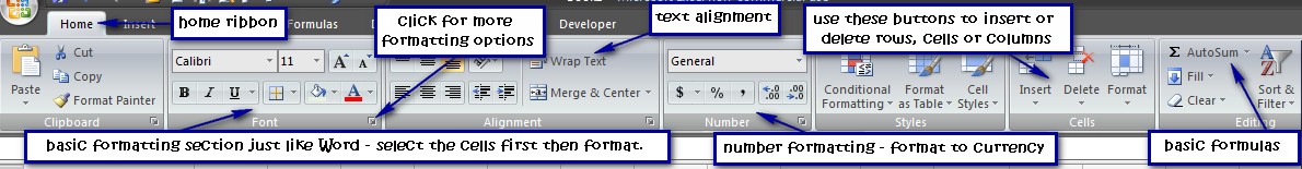
In the Total rows and Total column use the auto sum button (∑) to insert a formula that will add up your data as shown below.
Click in your first total row (for me it is B8), then click the auto sum button (top right corner of the home ribbon).
Next click in your first income cell above (for me it’s B3) and drag down all your income categories as shown below. Your cursor should look like a white cross as you drag down.
Press enter.
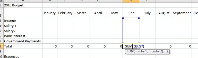
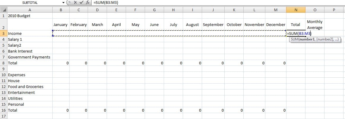
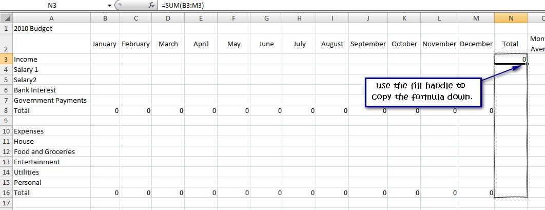
As with the headings click the fill handle and drag the formula across to December.
This copies the formula across all months. You can check that the formula is correct by double-clicking any of the formula cells and a highlighted rectangle will show you what is being calculated. Press ESC to get back out of the formula.
Do the same with the expenses Total row and the Total column as shown below.
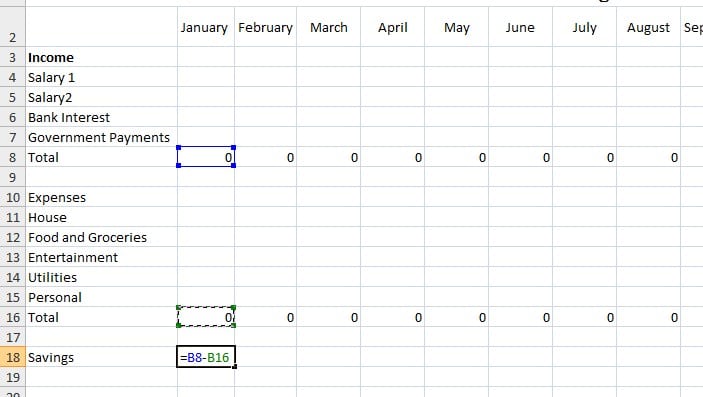
Skip a row and add a Savings row. This shows how much you’ve saved after taking your expense away from your income.
In the heading savings two cells under your total expenses. Then in the spreadsheet under January (in my example it’s B18), type the formula:
=total income – total expenses
In my case, I typed =B8-B16. You can click on the cells rather than typing the references (see below).
Then use the fill handle to copy this formula across.
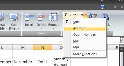
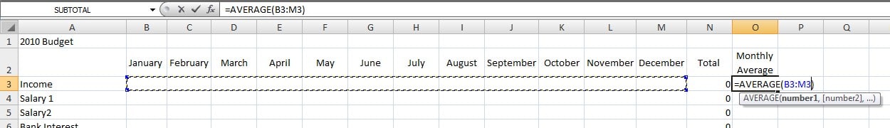
To calculate the Monthly Average, click under the Monthly Average Heading (O3 in my case), then click the drop-down arrow on the auto sum button to select average.
Select the cells from January to December (don’t include the total column), press enter and fill down, just as with the auto sum. Don’t worry about the #DIV/0! error, for now, that will be fixed once you enter some data.
Monthly averages are a good planning tool, especially if your earnings are irregular.
3. Format Your Budget Spreadsheet
Formatting your budget isn’t essential but is fun and it makes your spreadsheet easier to read which is always a good idea. You don’t want to miss something important because all the number swim together.
Formatting is very similar to most desktop applications like Word.
Formatting suggestions include:
- Start by formatting your heading. Select the rows A1 to O1 and click on the Merge and Centre button. Fancy up your heading as much as you like using the Font tools on the Home Ribbon.
- Use the Font tools in the Home Ribbon to format your month headings and income and expense headings.
- Use Bold and Fill to make the row totals and column totals stand out.
- Select all of the cells that will contain numbers and change the number format to currency.
- Add a border around your budget by selecting all the cells of your budget and choosing border – more (or Format: border for older versions) Click on outline and inside to add a border.
- Use the Fill Tool (the bucket) to lightly colour every second row to make the data easier to read.
Save As now and you will have a template that can be reused every year. Save As again to create a budget just for this year.
4. Test, Test, Test Your Spreadsheet
The budget decisions you make are only as good as the data you’re relying on. So you want to make sure there are no calculation errors in your spreadsheet.
Do this by entering easy data like $10 into various parts of your spreadsheet and making sure all the formulas calculate correctly.
5. Enter Data Into Your Spreadsheet
Now it’s time to fill in your budget.
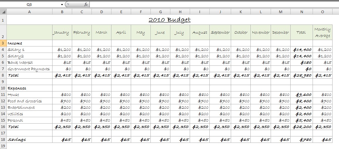
Type in expected income and expenses for each month. If you’ve been tracking your expenses, then use the information to fill in your budget.
If there are months where the income or expenses are zero, then type 0 – this will ensure that the average calculates properly. You will notice that the formulas change automatically as you add your data (tip: use the fill handle to copy values across your budget).
I’ve typed in some data to show you what it will look like, but you wouldn’t just type the same thing for each month.
If your car registration is due in January, for example, then your car rego category would only have a value under January, the rest of the year would be 0.
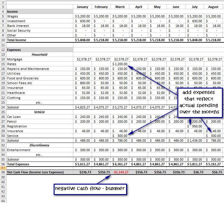
6. Examine Your Home Budget Spreadsheet
At this point, your budget is finished. How is it looking?
Check the savings row at the bottom of the budget. Is there an amount there? That is how much you can save each month, assuming your budget is accurate and you stick to your budget.
The months where the savings is zero, then you’re breaking even. And the months where there is a negative, you’ve spent more than you earn.
This might not necessarily be a bad things. I might be because a big bill came in that month. So compare it to the other months and look at the number in your Savings row under the Total column to see how you fair over the course of the whole year.
Here’s an example of a budget that I’ve finished formatting. The numbers are all made up.
In part two, I’ll show you how to set up the next part of your home budget spreadsheet Excel where you type actual income and expenses and use a formula to automatically calculate the variance between what was budgeted and what was actually earned/spent.


This is a really great how to! Super simple, yet incredibly effective. I know the Excel team would love to share your expertise with the community at the Excel page on Facebook. http://www.facebook.com/pages/Microsoft-Excel/89421301366
Cheers,
KIM
MSFT Office Outreach Team
You have inspired me to get my finances under control. You have made me very excited about Excel and my budget! I got a few surprises from looking at last year and can’t wait for the months to roll on to see this years progress.
Hi Rachel,
Hope your budgeting goes well.
I also get very excited about Excel – way too excited.
Melissa
I have created a website http://www.easy-budgeting.com that makes using an Excel budget planner simple and straightforward.
Excel is a great tool for budgeting but some people find it difficult or a bit overwhelming. I invested my time and knowledge to provide people with a solution to their budgeting needs without having to master Excel.
It’s helped 100’s of people worldwide and may be useful for your visitors.
Good luck, Rhys
Thanks Melisa – I thought I knew how to use excel, but you showed me heaps of different tricks there. Now I’m all set to start out the year right!
Ta Keldi, Good luck with your budgeting!